Advanced ploidy estimation
For instructions on installation and basic exploration steps, see Getting started.
[1]:
import isomut2py as im2
%matplotlib inline
Compiling C scripts...
Done.
Ploidy estimation from scratch
For a complete tutorial on how to perform ploidy estimation from a single bam file, we will be using the raw example dataset, that can be downloaded with:
[3]:
im2.examples.download_raw_example_data(path=exampleRawDataDir)
Downloading file from URL "http://genomics.hu/tools/isomut2py/isomut2py_raw_example_dataset.tar.gz" to isomut2py_download_dir/isomut2py_raw_example_dataset.tar.gz
File size: 528.5MiB
Downloading might take a while...
Download completed in 0 day(s), 2 hour(s), 49 min(s), 55 sec(s).
----------------------------------------
Extracting downloaded file to isomut2py_download_dir
Extracting completed in 0 day(s), 0 hour(s), 0 min(s), 7 sec(s).
And ploidy estimation settings can be loaded with:
examplePEResultsDir to a path where fairly large temporary files can be stored.[5]:
PEparam = im2.examples.load_example_ploidyest_settings(example_data_path=exampleRawDataDir,
                                                       output_dir=examplePEResultsDir)
We can generate a PloidyEstimator object and run the ploidy estimation with:
[6]:
PEst = im2.ploidyestimation.PloidyEstimator(**PEparam)
PEst.run_ploidy_estimation()
2018-11-15 12:47:24 - Ploidy estimation for file A.bam


        2018-11-15 12:47:24 - Preparing for parallelization...
                2018-11-15 12:47:24 - Defining parallel blocks ...
                2018-11-15 12:47:24 - Done

        2018-11-15 12:47:24 - (All output files will be written to ../Documents/isomut2py_example_data/PE_example_results_20181114)

        2018-11-15 12:47:24 - Generating temporary files, number of blocks to run: 107
        2018-11-15 12:47:24 - Currently running:  1 2 3 4 5 6 7 8 9 10 11 12 13 14 15 16 17 18 19 20 21 22 23 24 25 26 27 28 29 30 31 32 33 34 35 36 37 38 39 40 41 42 43 44 45 46 47 48 49 50 51 52 53 54 55 56 57 58 59 60 61 62 63 64 65 66 67 68 69 70 71 72 73 74 75 76 77 78 79 80 81 82 83 84 85 86 87 88 89 90 91 92 93 94 95 96 97 98 99 100 101 102 103 104 105 106 107

        2018-11-15 12:47:55 - Temporary files created, merging, cleaning up...

        2018-11-15 12:47:55 - Estimating haploid coverage by fitting an infinite mixture model to the coverage distribution...

                2018-11-15 12:59:18 - Raw estimate for the haploid coverage: 27.046445720783716

        2018-11-15 12:59:18 - Fitting equidistant Gaussians to the coverage distribution using the raw haploid coverage as prior...

                2018-11-15 13:06:27 - Parameters of the distribution are saved to: ../Documents/isomut2py_example_data/PE_example_results_20181114/GaussDistParams.pkl

                2018-11-15 13:06:27 - Final estimate for the haploid coverage: 32.45404396554027

        2018-11-15 13:06:27 - Estimating local ploidy using the previously determined Gaussians as priors on chromosomes:  I II III IV V VI VII VIII IX X XI XII XIII XIV XV XVI

        2018-11-15 13:10:14 - Generating final bed file...


        2018-11-15 13:10:15 - Generating HTML report...


2018-11-15 13:10:49 - Ploidy estimation finished. (0 day(s), 0 hour(s), 23 min(s), 24 sec(s).)
The ploidy estimation pipeline consists of the following main steps:
- A temporary pileup file is generated from the original bam file which is scanned with a moving average method to determine the reference allele frequency and the local average coverage for a set of investigated positions. This is performed in a highly parallelized manner, on short regions of the genome. Information collected for the genomic positions are temporarily saved to a set of intermediate files (one for each chromosome).
- The average coverage of the haploid regions is estimated. This is achieved by fitting a many-component (20) Gaussian mixture model 10 times to the coverage distribution determined from the intermediate files. Using specific statistics of the parameters of the fitted distributions, an estimate for the haploid coverage is obtained. This whole step can be completely skipped by supplying an estimate value in the
user_defined_hapcovattribute of the PloidyEstimator object. (If one has a reasonable idea about the haploid coverage (for example by checking sequencing results with a genome viewer), it is generally a good idea to set theuser_defined_hapcovto this value to save time. For a strictly non-haploid genome, the haploid coverage is defined as the half of the diploid, the third of the triploid, etc. coverages.) - A seven component Gaussian mixture model is fitted to the coverage distribution with equidistant centers. The estimated (or user-defined) haploid coverage and its products with whole numbers are used as prior for the centers of the components, allowing the identification of seven distinct ploidies.
- The seven component fitted distribution is used as prior to determine the ploidy of each genomic position in the intermediate files.
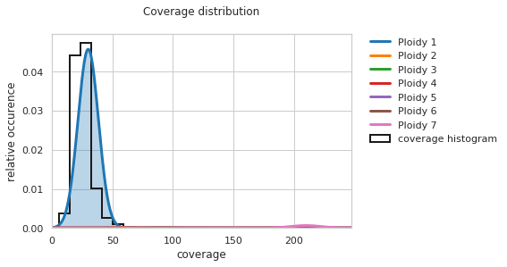
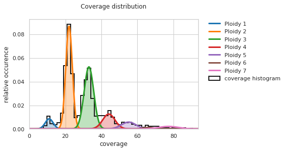
Thus the actual ploidy estimation largely depends on how accurately the seven component model fits the raw coverage distribution. It is good practice to check this by plotting them both on the same figure with:
[7]:
f = PEst.plot_coverage_distribution()
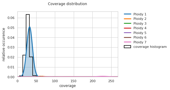
Given that the currently investigated sample is an almost fully haploid genome, having a single peak on the figure for the “Ploidy 1” curve is promising. However, the center of this curve is slightly shifted to the right.
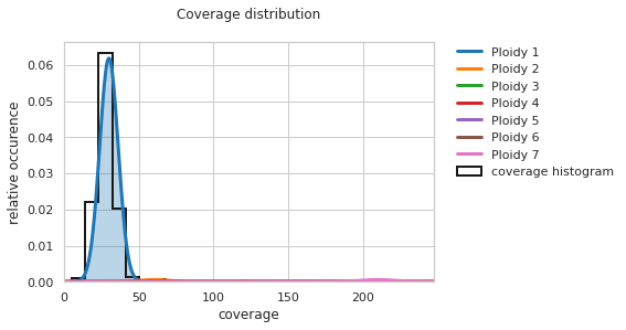
If you are unhappy with the fit, estimate the haploid coverage manually, and try refitting the seven component model with:
[8]:
PEst.fit_gaussians(estimated_hapcov = 25)
[9]:
f = PEst.plot_coverage_distribution()
Naturally, you will need to rerun the final step of the ploidy estimation with the improved fit:
[10]:
PEst.PE_on_whole_genome()
I II III IV V VI VII VIII IX X XI XII XIII XIV XV XVI
Visualizing karyotypes
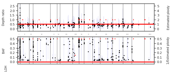
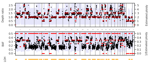
To plot the results of ploidy estimation, isomut2py provides two function. A fairly concise summary of the results can be plotted with:
binsize, overlap and min_PL_length are set to accomodate the plotting of large (human) genomes, thus for our current case, they should be adjusted to allow for a more easily interpretable figure. The value of overlap must always be smaller than binsize. These are used as shift- and windowsizes (respectively) for a moving average method that condenses the data to plottable points. The smaller their values are, the more points will appear on the
figure, but the longer it will take to plot. Similary, min_PL_length controls the minimal length of a region with an unique ploidy to be plotted on the graph.[11]:
f = PEst.plot_karyotype_summary(binsize=100, overlap=10, min_PL_length=300)
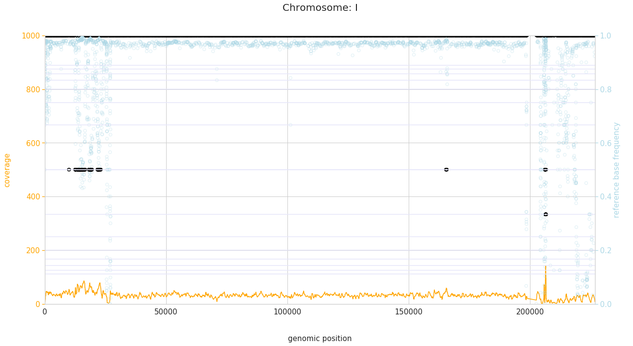
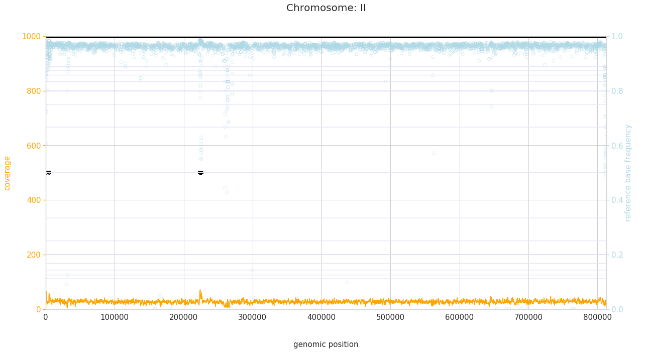
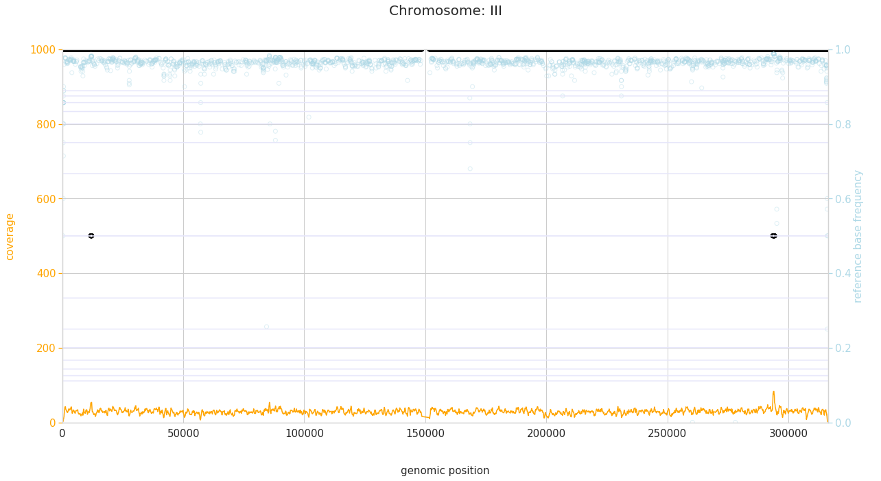
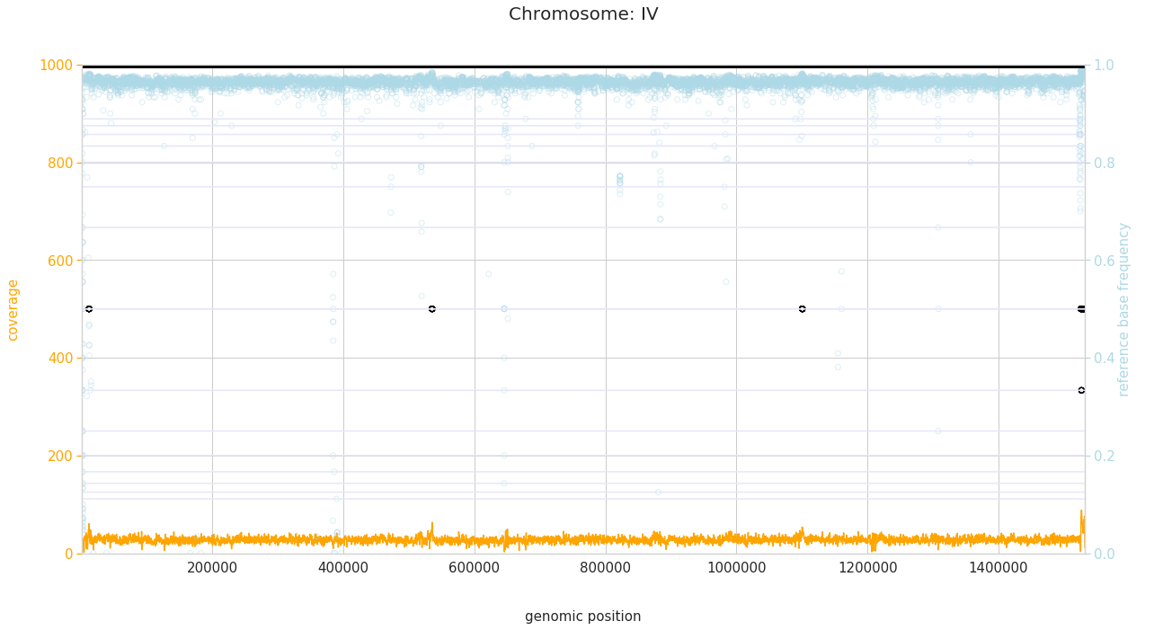
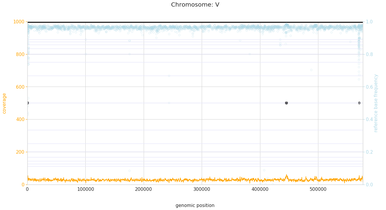
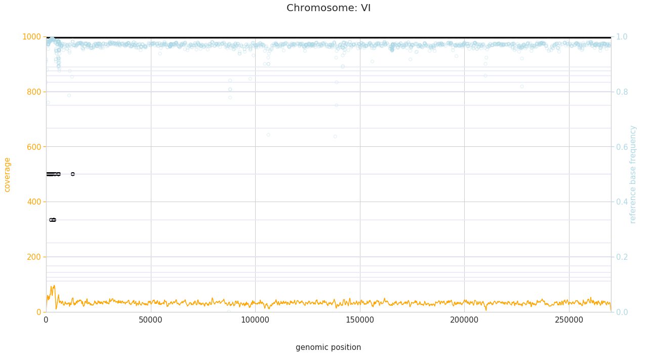
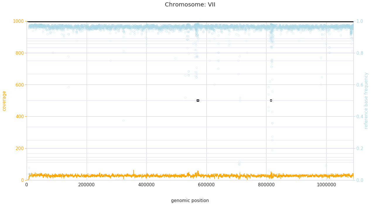
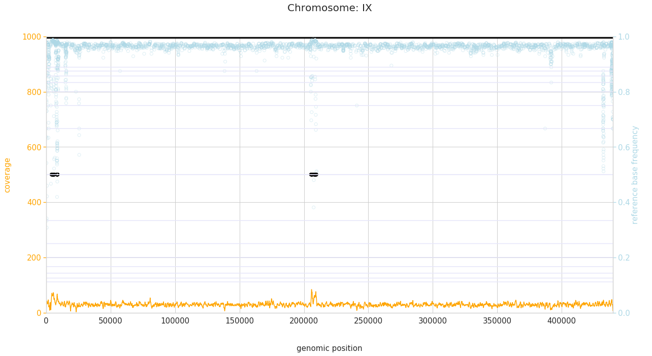
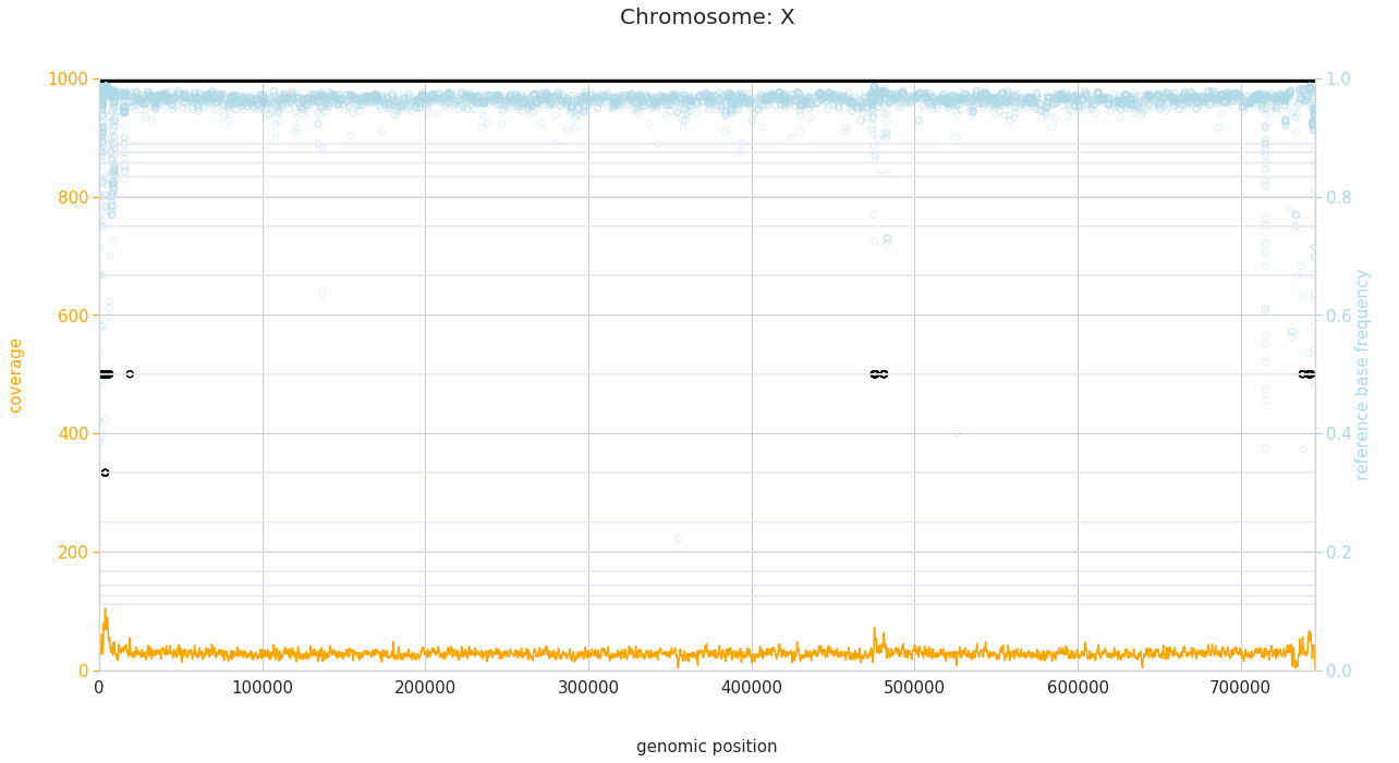
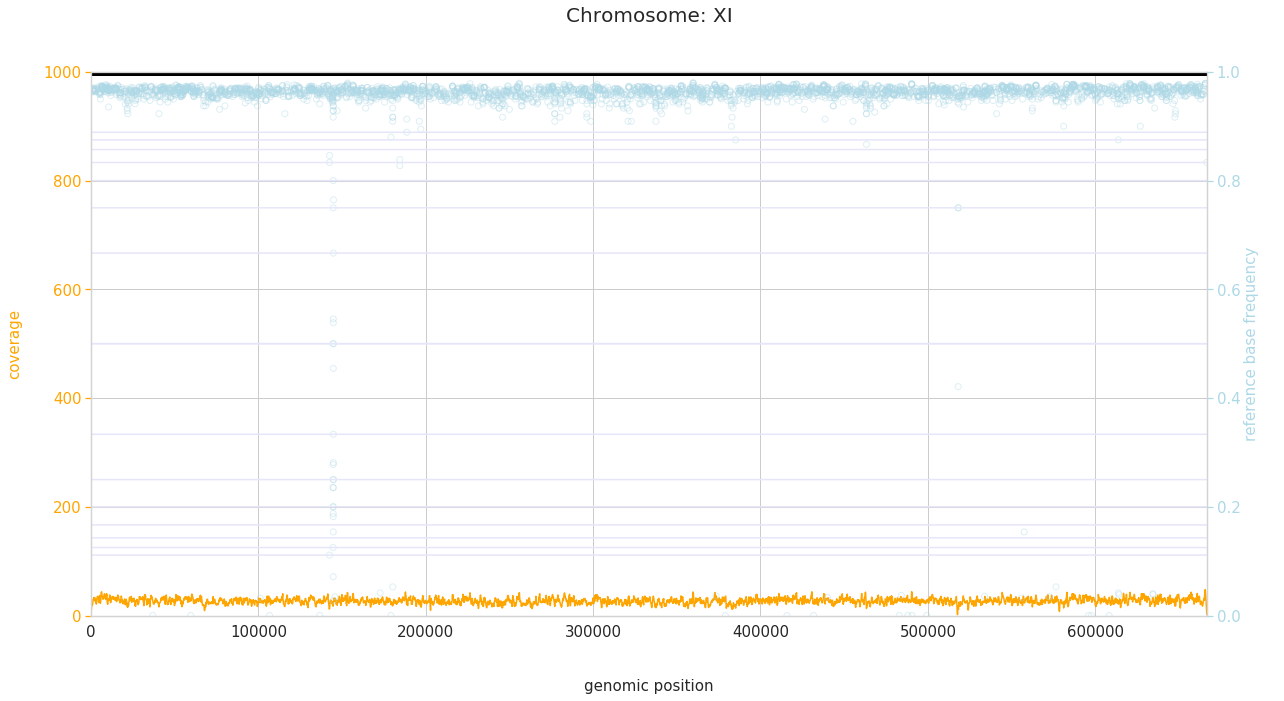
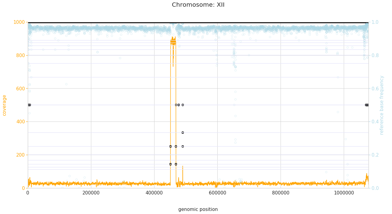
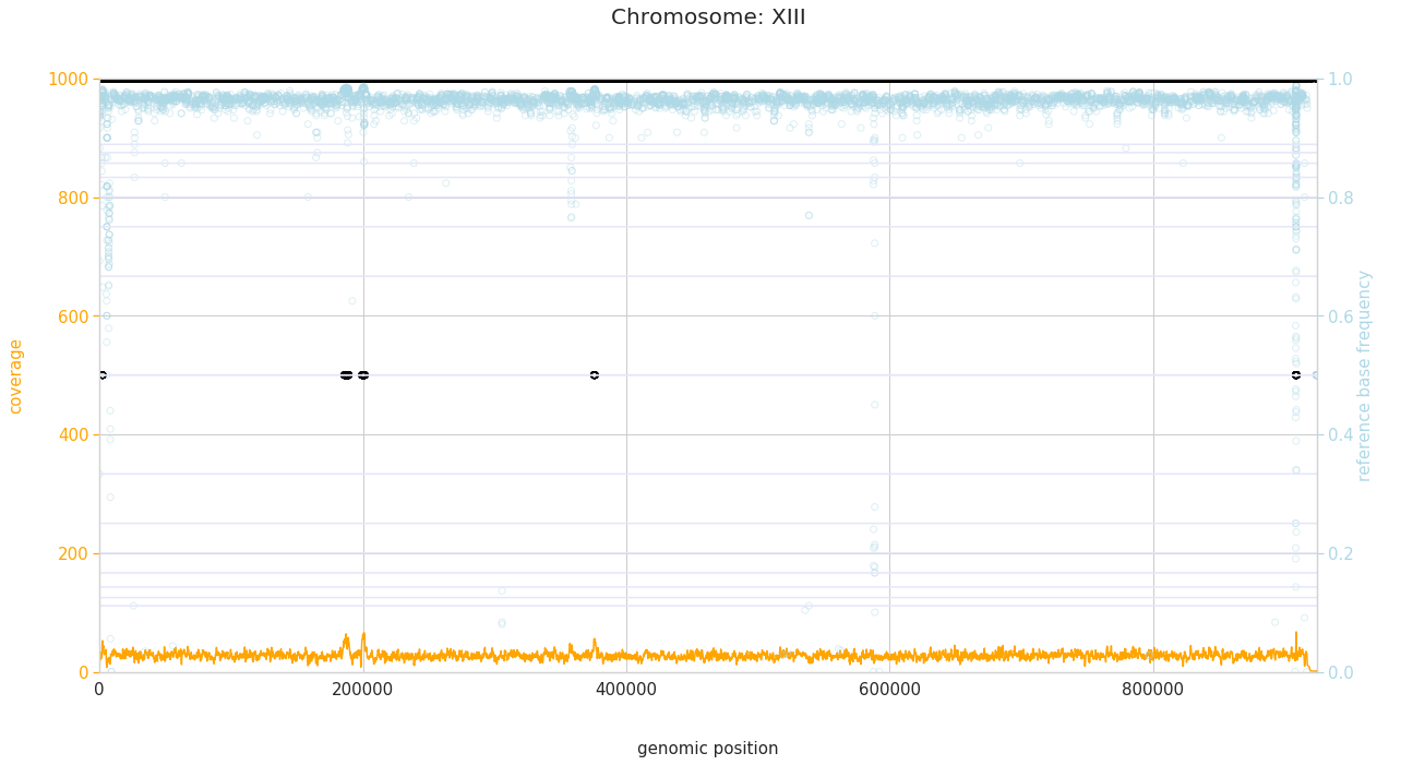
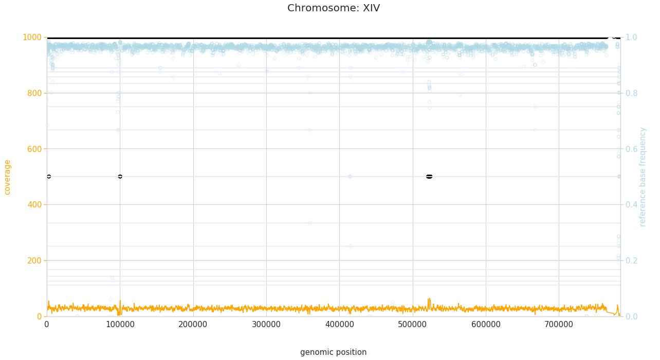
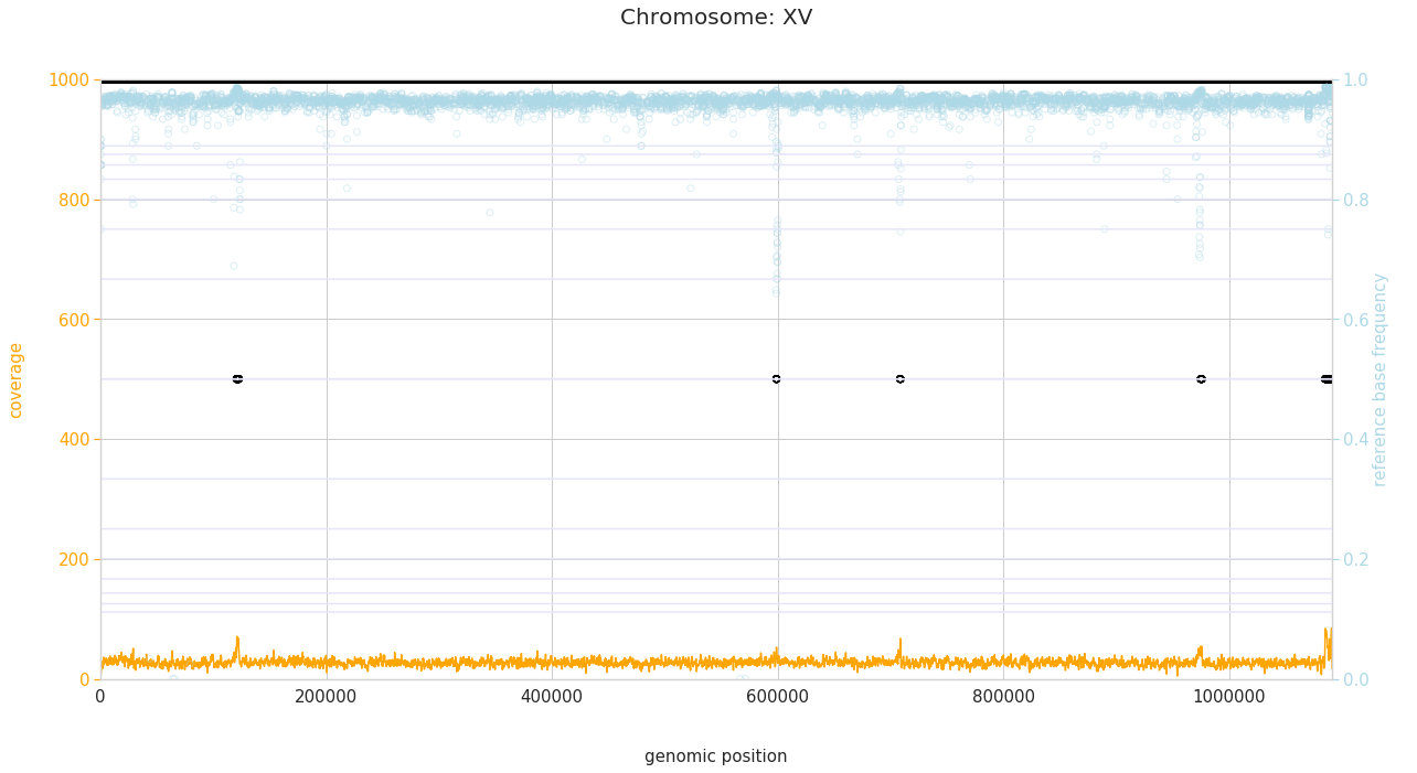
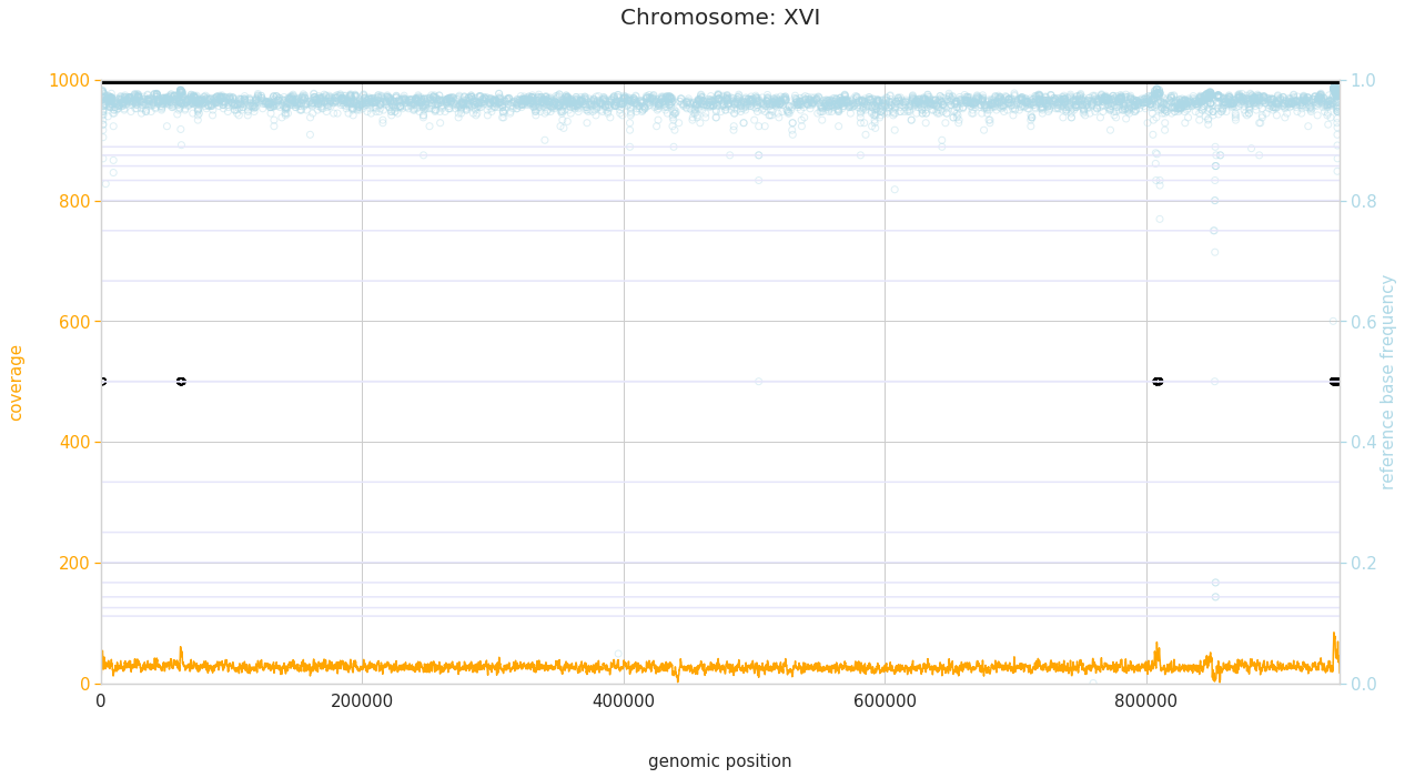
A more detailed plot of individual chromosomes can be generated with:
[12]:
f = PEst.plot_karyotype_for_all_chroms()

Comparing samples
A naive karyotype comparison of the samples is incorporated in isomut2py. However, we suggest using this option more as an exploratory step rather than a chosen tool for the accurate detection of copy number variations.
As a necessary first step, the ploidy estimation for another sample has to be performed. This can be easily achieved by slightly modifying the code used above:
[5]:
PEparam_2 = im2.examples.load_example_ploidyest_settings(example_data_path=exampleRawDataDir,
                                                       output_dir=examplePEResultsDir_2)
[6]:
PEst_2 = im2.ploidyestimation.PloidyEstimator(**PEparam_2)
PEst_2.bam_filename = 'B.bam'
[7]:
PEst_2.run_ploidy_estimation(user_defined_hapcov=25)
2018-11-15 14:35:37 - Ploidy estimation for file B.bam


        2018-11-15 14:35:37 - Preparing for parallelization...
                2018-11-15 14:35:37 - Defining parallel blocks ...
                2018-11-15 14:35:37 - Done

        2018-11-15 14:35:37 - (All output files will be written to ../Documents/isomut2py_example_data/PE_example_results_20181114_B)

        2018-11-15 14:35:37 - Generating temporary files, number of blocks to run: 107
        2018-11-15 14:35:37 - Currently running:  1 2 3 4 5 6 7 8 9 10 11 12 13 14 15 16 17 18 19 20 21 22 23 24 25 26 27 28 29 30 31 32 33 34 35 36 37 38 39 40 41 42 43 44 45 46 47 48 49 50 51 52 53 54 55 56 57 58 59 60 61 62 63 64 65 66 67 68 69 70 71 72 73 74 75 76 77 78 79 80 81 82 83 84 85 86 87 88 89 90 91 92 93 94 95 96 97 98 99 100 101 102 103 104 105 106 107

        2018-11-15 14:36:06 - Temporary files created, merging, cleaning up...

        2018-11-15 14:36:06 - Collecting data for coverage distribution, using user-defined haploid coverage (25)...

        2018-11-15 14:36:06 - Fitting equidistant Gaussians to the coverage distribution using the raw haploid coverage as prior...

                2018-11-15 14:43:14 - Parameters of the distribution are saved to: ../Documents/isomut2py_example_data/PE_example_results_20181114_B/GaussDistParams.pkl

                2018-11-15 14:43:14 - Final estimate for the haploid coverage: 29.99889722813764

        2018-11-15 14:43:14 - Estimating local ploidy using the previously determined Gaussians as priors on chromosomes:  I II III IV V VI VII VIII IX X XI XII XIII XIV XV XVI

        2018-11-15 14:47:40 - Generating final bed file...


        2018-11-15 14:47:41 - Generating HTML report...


2018-11-15 14:48:13 - Ploidy estimation finished. (0 day(s), 0 hour(s), 12 min(s), 35 sec(s).)
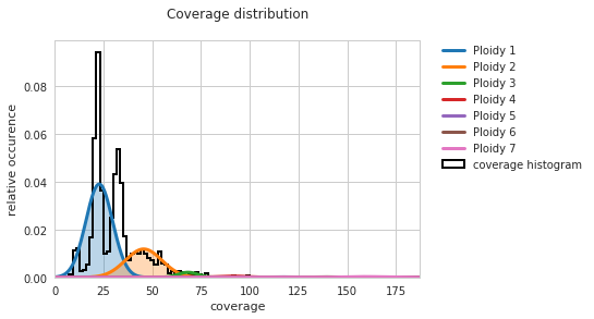
[8]:
f = PEst_2.plot_coverage_distribution()
Now the comparison can be done in a single step with:
[13]:
PEst.compare_with_other(PEst_2)
2018-11-15 14:56:17 - Comparing regions of different ploidies in detail

        2018-11-15 14:56:17 - Number of intervals to check: 2

                2018-11-15 14:56:17 - Currently running: 1 2

        2018-11-15 14:56:17 - Differing genomic intervals with quality scores saved to file ../Documents/isomut2py_example_data/PE_example_results_20181114A_VS_B_COMP.bed


2018-11-15 14:56:17 - Comparison finished.
The comparison results stored in the above file can be checked with:
[17]:
!cat ../Documents/isomut2py_example_data/PE_example_results_20181114/A_VS_B_COMP.bed
chrom   intStart        intEnd  ploidy1 ploidy2 LOH1    LOH2    intLength       quality
VII     289734  291768  1       3       0       0       2034    619987021.8068602
XII     1072935 1075050 2       1       0       0       2115    0.8403883817503438
Correcting bad fits, loading fitted coverage distributions
As the distribution fitting is the most time consuming part of the ploidy estimation, it can be useful to load an already fitted distribution that we can work with. The above used ploidy estimation pipeline automatically saves the parameters of the fitted distribution to a file in the output directory, so these can be easily reused.
As an example, we will be using the already prepared files in the example dataset. (For download instructions, see Getting started.)
[3]:
PEparam_3 = im2.examples.load_preprocessed_example_ploidyest_settings(example_data_path=exampleDataDir)
[4]:
PEst_3 = im2.ploidyestimation.PloidyEstimator(**PEparam_3)
[6]:
PEst_3.load_cov_distribution_parameters_from_file(PEst_3.output_dir + 'GaussDistParams_incorrect.pkl')
[7]:
f = PEst_3.plot_coverage_distribution()
This is obviously a highly incorrect fit for this data. In cases like this, the above described procedure can be followed: the haploid coverage should be estimated manually (essentially by looking at the position of the first peak of the above histogram), and the fitting rerun with this user-defined value:
[9]:
PEst_3.fit_gaussians(estimated_hapcov = 11)
[32]:
f = PEst_3.plot_coverage_distribution()
And finally, ploidy estimation can be rerun with the now correct prior distribution with:
[6]:
PEst_3.PE_on_whole_genome()
1 2 3 4 5 6 7 8 9 10 11 12 13 14 15 16 17 18 19 20 21 22 X Y
[8]:
f = PEst_3.plot_karyotype_summary()
Using estimated ploidies as input for mutation detection
Once the ploidy estimation has been performed as described, we can use this information to fine-tune mutation detection. Mutation calling is run on diploid genomes by default, however, when analysing non-diploid genomes or genomes with largely varying ploidies (as shown above), it can be useful to determine the ploidy more precisely. (This is important because the alternate allele frequency in mutated positions largely depends on the local ploidy.)
If the analysed organism (all of the samples in the sample set) has a constant ploidy different from 2 (for example, a fully haploid genome), its value can be simply set with:
mutDet = im2.mutationcalling.MutationCaller()
mutDet.constant_ploidy = 1
(For basic mutation calling, see Getting started.)
However, in cases when some of the analysed samples have varying ploidy along the length of the genome (for example, aneuploid cell lines), the local ploidy can be uniquely defined for each sample and each genomic position in a bed file.
As a best practice, we suggest performing the above ploidy estimation on the starting clones in a sample set. This creates a separate ploidy bed file for each sample group derived from the starting clones. These can be assigned to specific samples with (make sure to provide valid paths to the bed files):
[8]:
im2.format.generate_ploidy_info_file(sample_groups=[['S1.bam', 'S2.bam', 'S3.bam'],
                                                    ['S4.bam', 'S5.bam', 'S6.bam', 'S7.bam']],
                                     group_bed_filepaths=['path_to_S1_ploidy.bed', 'path_to_S4_ploidy.bed'],
                                     filename='ploidy_info_file_for_test_set.txt')
The above function generates a ploidy info file to the path specified by filename:
[9]:
!cat ploidy_info_file_for_test_set.txt
#file_path      sample_names_list
path_to_S1_ploidy.bed_im2format S1.bam, S2.bam, S3.bam
path_to_S4_ploidy.bed_im2format S4.bam, S5.bam, S6.bam, S7.bam
Now this file can be supplied to the mutation detection object with:
mutDet.ploidy_info_file = "ploidy_info_file_for_test_set.txt"
(Make sure to set the complete path to the file.)
For all samples in the dataset that are not included in the ploidy info file, the constant ploidy set with the constant_ploidy attribute will be used (default: 2). This is also true for any genomic regions that were not specified in the bed files.