Further analysis, visualization
Once a basic set of mutations has been recovered for the analysed sample set, one can proceed with additional visualization and postprocessing steps. These are demonstrated here.
Recovering mutations
There are three options to produce a dataframe which stores all the mutations present in the investigated sample set:
- Run the
isomut2pymutation detection pipeline. (See Getting started.) - Load the list of mutations previously detected by
isomut2py. - Import mutations detected by external tools. (See Importing external mutations.)
For now, we will use the second option with a dataframe provided in the example dataset. (For instructions on download, see Getting started.) The reference genome used for this set of mutations can be found in the same directory.
[73]:
import pandas as pd
import isomut2py as im2
%matplotlib inline
[74]:
exampleDataDir='/nagyvinyok/adat83/sotejedlik/orsi/'
[81]:
mutations_df = pd.read_csv(exampleDataDir+'isomut2py_example_dataset/Vizualisation/mutations_dataframe.csv', sep='\t')
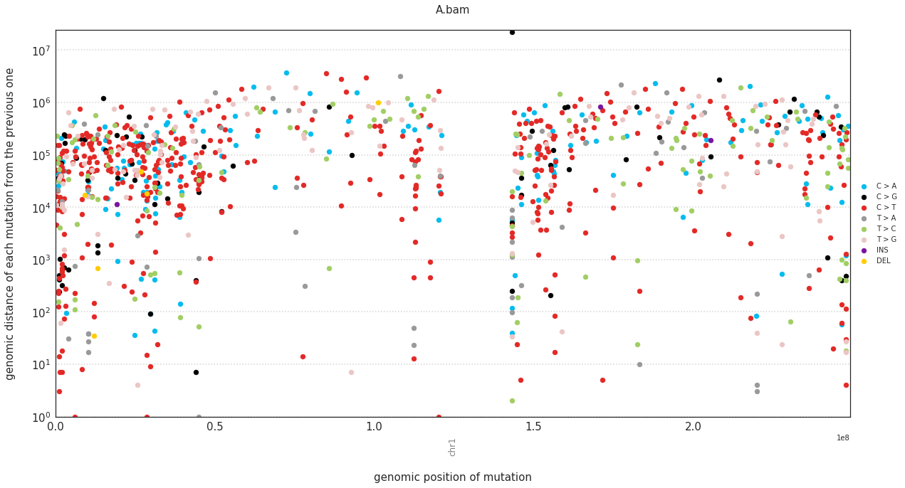
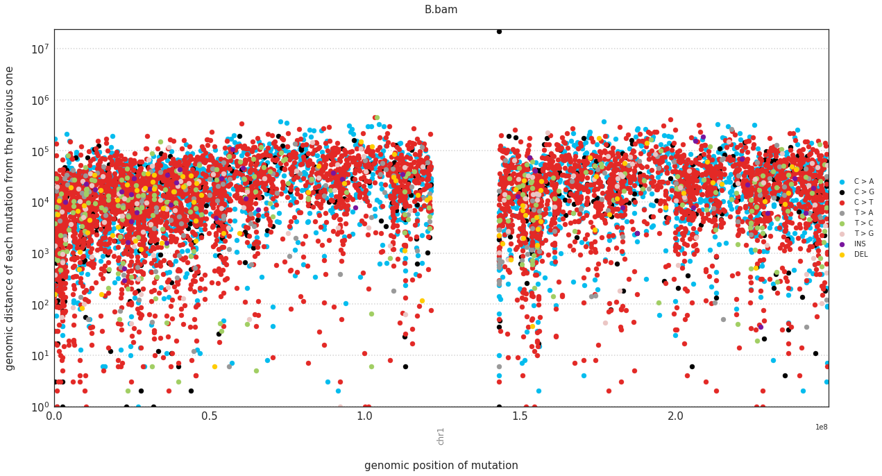
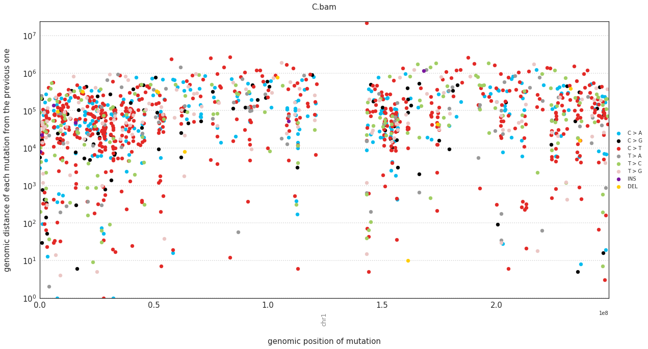
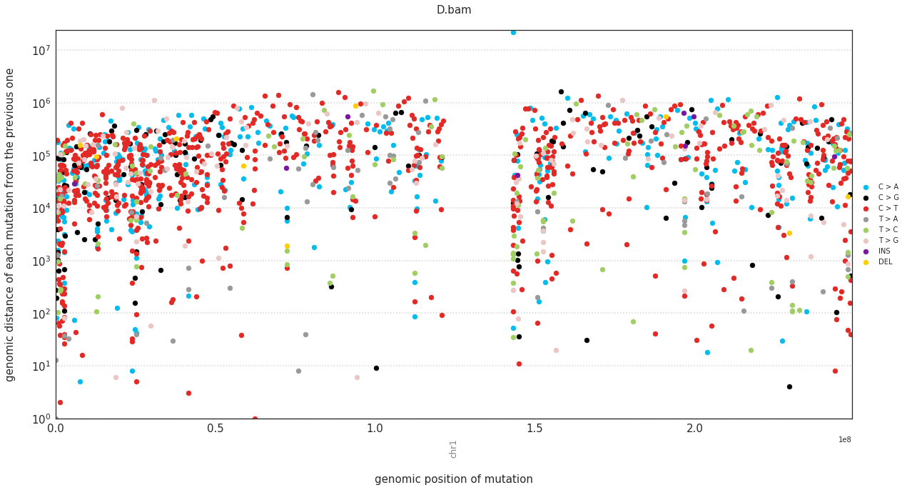
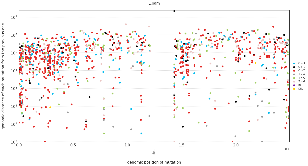
Plotting mutations on rainfall plots
(To simply plot the number of mutations in each sample, see Getting started.)
In a rainfall plot, the horizontal axis represents the genomic position of a mutations, while the vertical axis shows the distance from the previous mutation. Thus mutational clusters appear on the bottom part of the rainfall plots as a cluster of dots.
These can be plotted with:
[86]:
f = im2.plot.plot_rainfall(mutations_dataframe=mutations_df,
                           ref_fasta=exampleDataDir+'isomut2py_example_dataset/Vizualisation/chr1.fa')
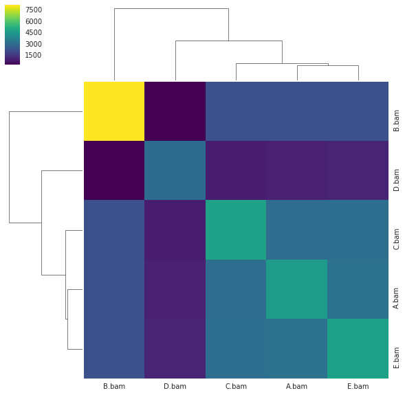
Plotting a simple hierarchical clustering of the samples
A naive hierarchical clustering of the analysed samples based on the number of shared mutations can be plotted with:
[88]:
f = im2.plot.plot_hierarchical_clustering(mutations_dataframe=mutations_df)
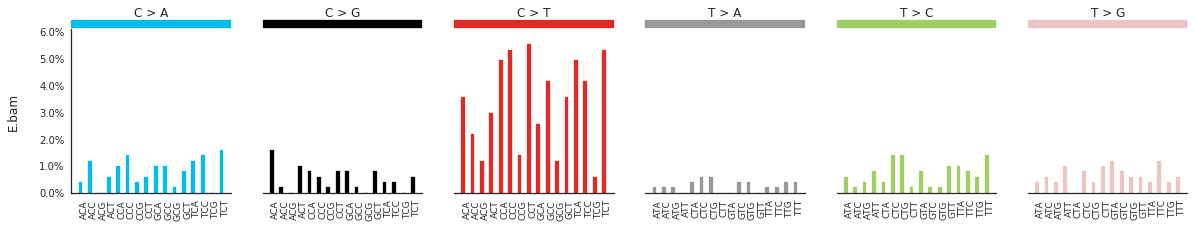
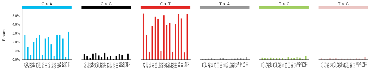
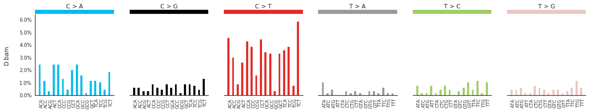
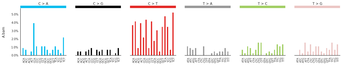
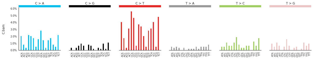
Plotting the spectra of mutations
The spectra of different mutation types are defined in this paper.
To calculate and plot the spectra of SNVs in the samples, use:
[83]:
SNV_spectra = im2.postprocess.calculate_SNV_spectrum(ref_fasta=exampleDataDir+'isomut2py_example_dataset/Vizualisation/chr1.fa',
                                                     mutations_dataframe=mutations_df)
[85]:
f = im2.plot.plot_SNV_spectrum(spectrumDict=SNV_spectra, normalize_to_1=True)
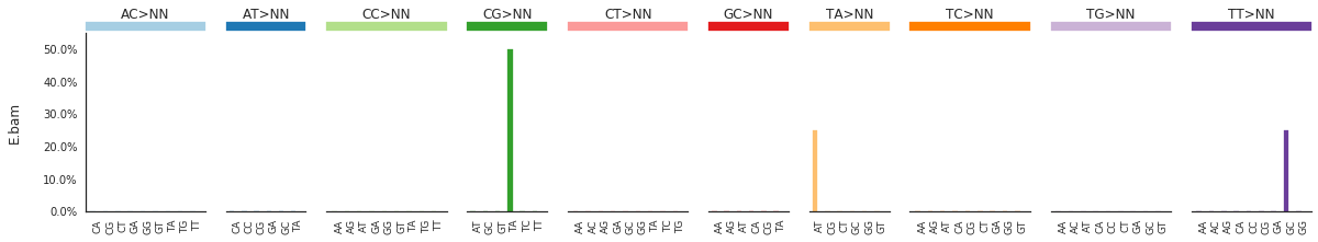
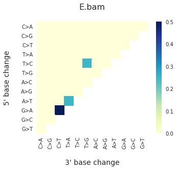
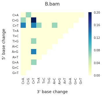
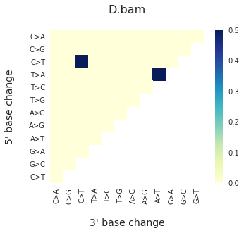
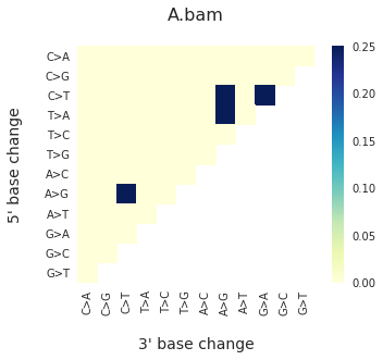
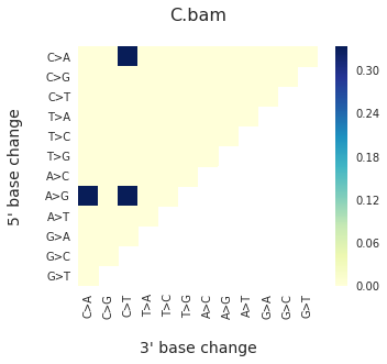
To get the DNV spectra in a linear and a heatmap format, use:
[89]:
DNVspectra = im2.postprocess.calculate_DNV_spectrum(mutations_dataframe=mutations_df)
DNVmatrix = im2.postprocess.calculate_DNV_matrix(mutations_dataframe=mutations_df)
[90]:
f = im2.plot.plot_DNV_spectrum(spectrumDict=DNVspectra, normalize_to_1=True)
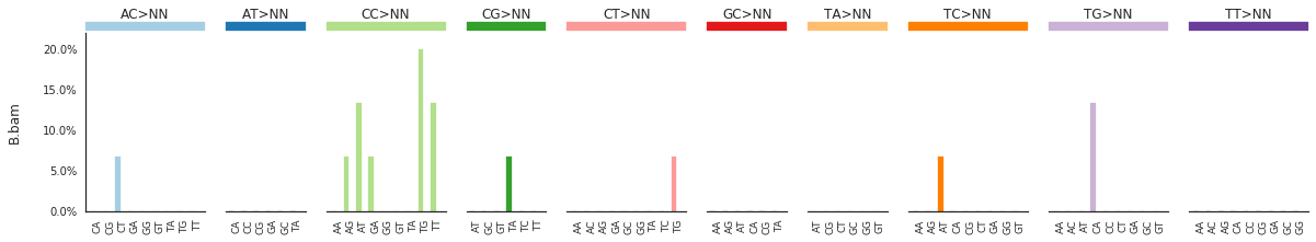
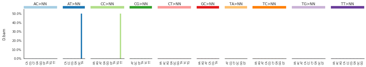
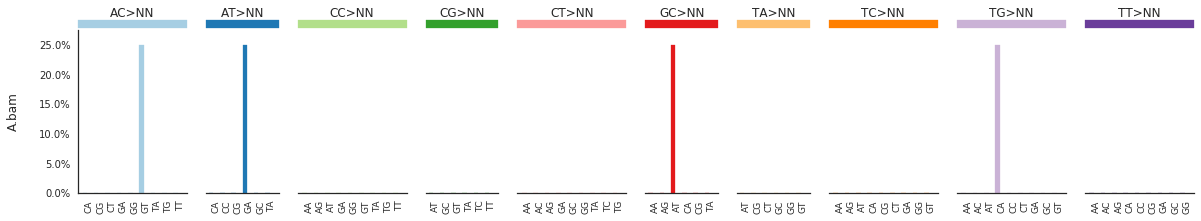
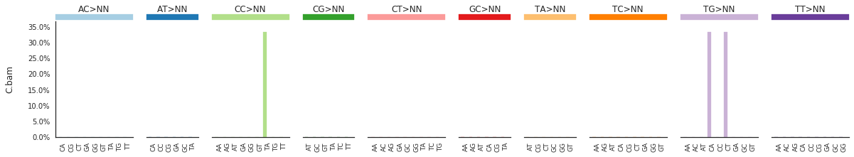
[91]:
f = im2.plot.plot_DNV_heatmap(matrixDict=DNVmatrix, normalize_to_1=True)
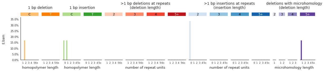
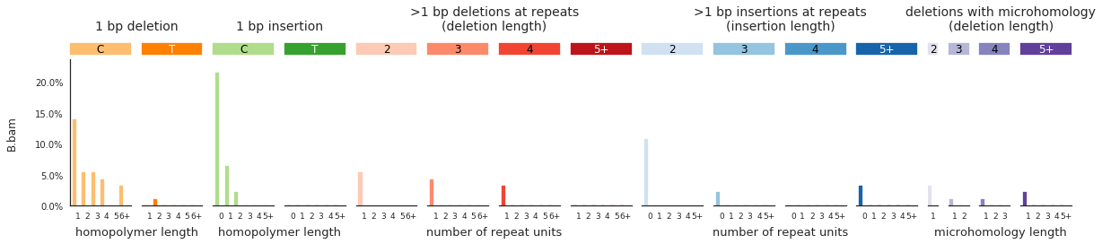
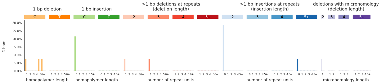
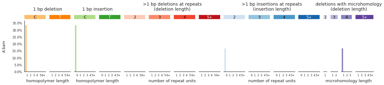
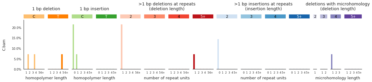
And finally, to get indel spectra, use:
[92]:
IDspecra = im2.postprocess.calculate_indel_spectrum(ref_fasta=exampleDataDir+'isomut2py_example_dataset/Vizualisation/chr1.fa',
                                                     mutations_dataframe=mutations_df)
[93]:
f = im2.plot.plot_indel_spectrum(spectrumDict=IDspecra, normalize_to_1=True)
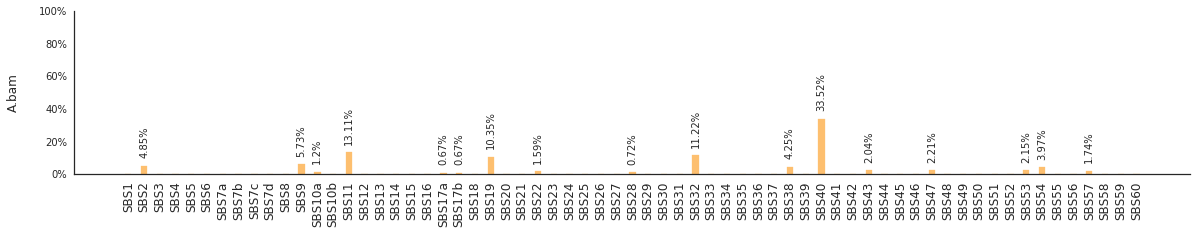
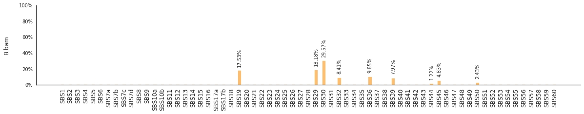
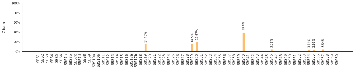
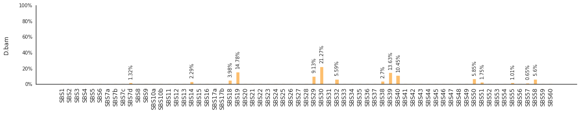
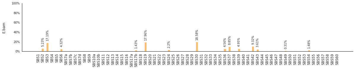
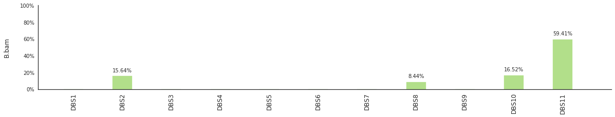
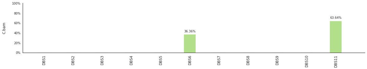
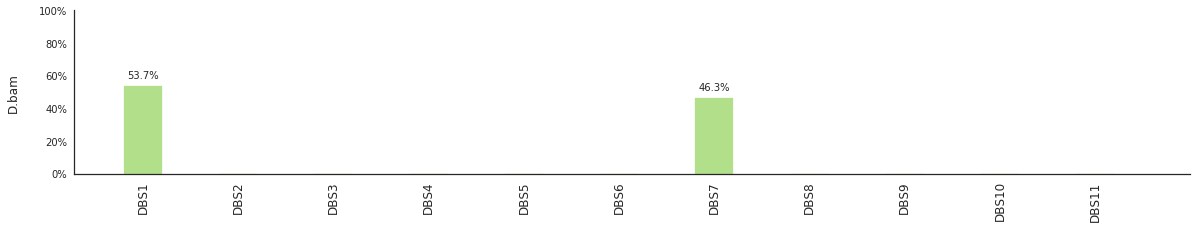
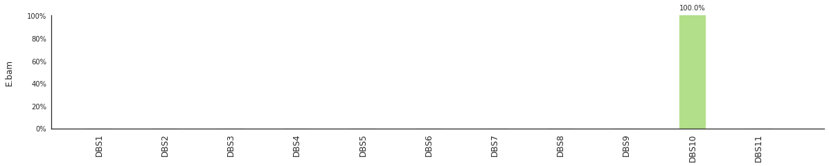
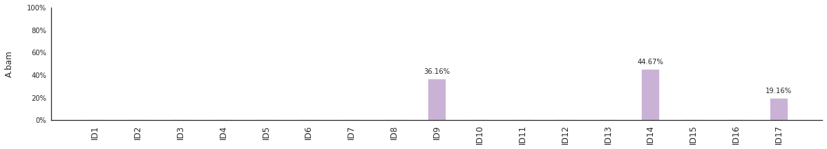
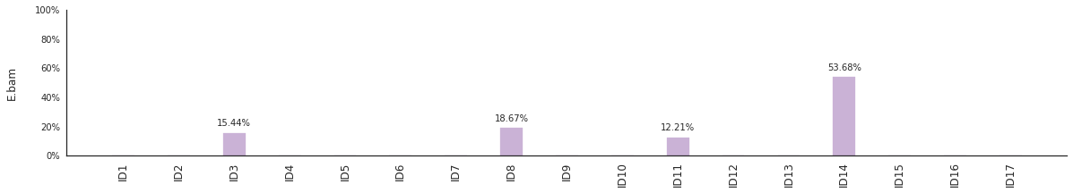
Decomposing mutational spectra to reference signatures
Using the consensus signatures described in the paper above, we can decompose mutational spectra to weighted contributions of the reference signatures. These can be achieved with:
[94]:
f = im2.postprocess.decompose_SNV_spectra(SNVspectrumDict=SNV_spectra)
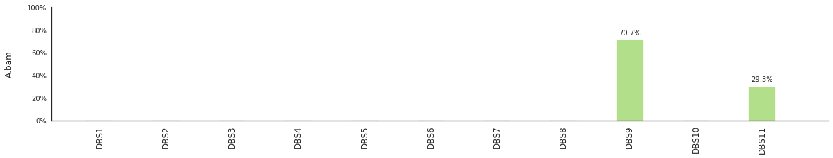
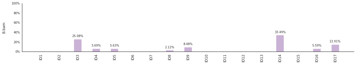
[95]:
f = im2.postprocess.decompose_DNV_spectra(DNVspectrumDict=DNVspectra)
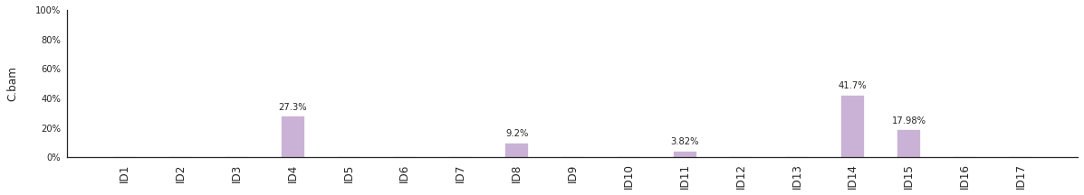
[96]:
f = im2.postprocess.decompose_indel_spectra(IDspectrumDict=IDspecra)
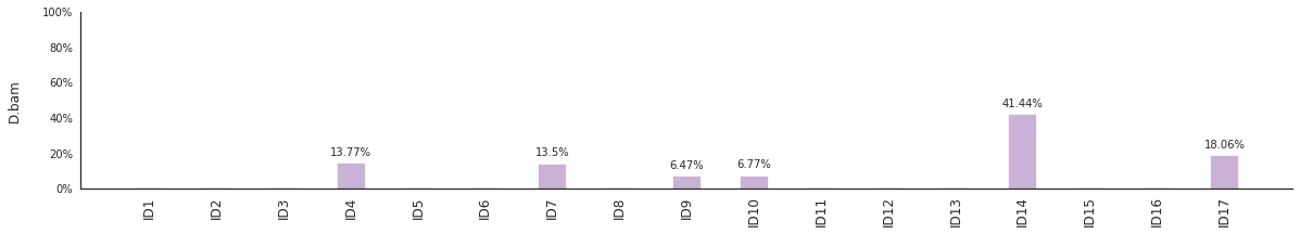
The set of reference signatures used can be modified by setting the argument signatures_file in the above functions. The set of mutations included in the decomposition can be set by using the use_signatures and ignore_signatures arguments.